
In the Nodi desktop version, you can run analysis (CAE) on modeled shapes directly from the node editor. At the core of this analysis capability is meshless analysis (Immersed FEM: immersed boundary finite element method).
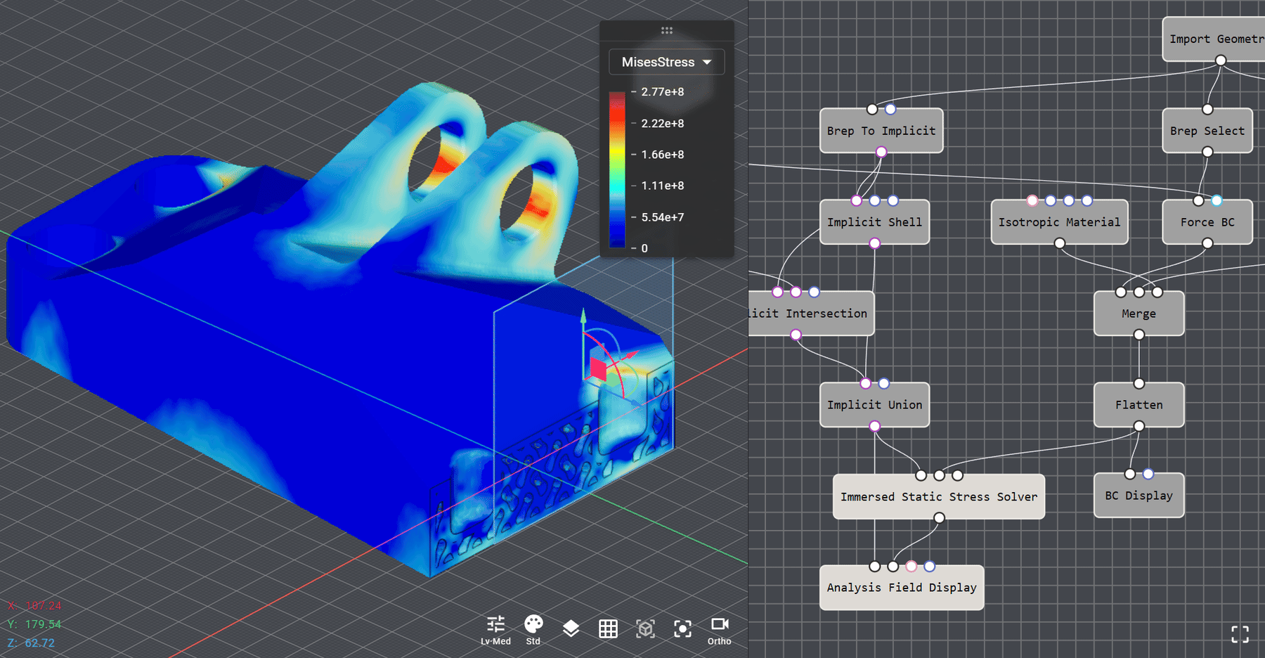
This article introduces how meshless analysis works, its affinity with Implicit modeling, examples of structural, fluid, and thermal analysis, and its application to topology optimization.
Meshless Analysis (Immersed FEM) in Nodi
Nodi’s analysis solver is a 3D FEM solver based on an implicit function representation of shapes. What makes it fundamentally different from typical FEM solvers is that it does not create a mesh fitted to the shape being analyzed.
Roughly speaking, it works as follows:
- A uniform structured grid (8-node hexahedral elements) is automatically generated over a box-shaped domain enclosing the target shape
- The shape is sampled at each grid node as a signed distance field (SDF), storing “how far inside the shape” each point is as a distance value
- Elements intersected by the shape’s surface are computed considering only their interior region
- Boundary conditions (fixtures, loads, temperatures, etc.) are applied not to mesh nodes, but to surfaces or regions placed to cover the shape’s boundary
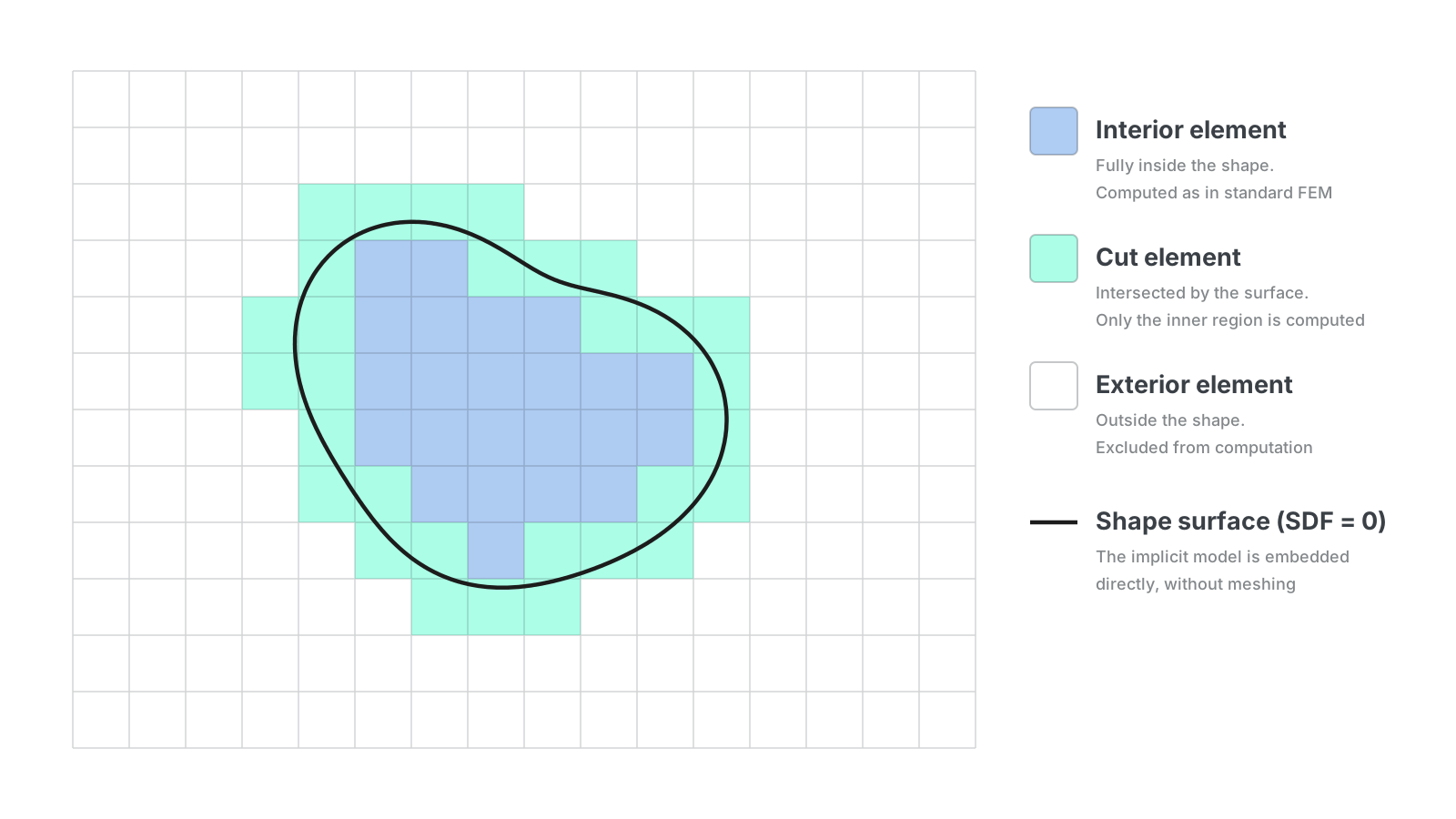
In other words, the shape (SDF) and the computational grid (structured grid) are completely decoupled, and there is no step where the user creates a mesh. This kind of approach is generally categorized as non-boundary-conforming (unfitted) analysis, a family that includes methods such as Immersed FEM, the immersed boundary method, and CutFEM.1
Background: The Meshing Problem in Classical FEM
Traditional FEM requires creating a mesh that conforms to the shape’s boundary before analysis can begin. As anyone who has used CAE in practice knows, this meshing step is the biggest bottleneck in the analysis workflow.
- Mesh quality determines analysis accuracy: distorted elements and elements with poor aspect ratios degrade accuracy and convergence, requiring careful mesh control around local features such as fillets and thin walls
- CAD cleanup as preprocessing: getting a shape through the mesher often requires shape repair such as removing tiny faces
- Remeshing on every design change: even a small change to the shape requires remeshing, creating major friction in the design–analysis iteration loop
In the context of DfAM (Design for Additive Manufacturing), this problem becomes even more severe. For shapes with complex internal structures such as TPMS lattices, creating a boundary-conforming mesh is practically infeasible in the first place. Even if a mesh could be created, the element count explodes, making it impossible to casually run analysis inside a design loop.
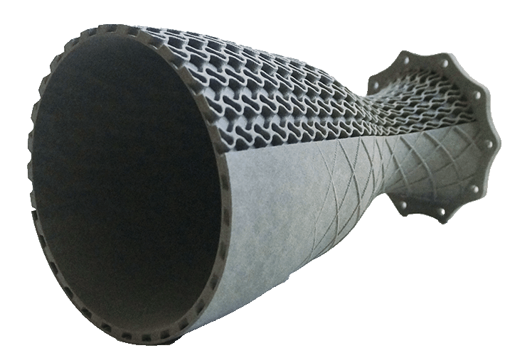
Meshless analysis (Immersed FEM) avoids this problem at its root. Since the background grid is a uniform box grid independent of the shape, grid generation never fails no matter how complex the shape is, and the analysis can always be run.
Affinity with Implicit Modeling
Nodi supports Implicit modeling, introduced in a previous article. Implicit modeling represents shapes as implicit functions, and this is an exceptionally good match for meshless analysis.
This is because the information Immersed FEM asks of a shape is “whether a point in space is inside or outside the shape (and how far it is from the boundary)” — exactly the question that the shape representation of Implicit modeling (the SDF) is built to answer.
- Shapes created with Implicit modeling become analysis input without any meshing step (there is no intermediate meshing or repair stage)
- Shapes for which meshing is impractical, such as TPMS lattices and porous structures, can be analyzed as they are
When these properties of Implicit modeling and Immersed FEM come together within a procedural, node-graph-based workflow, the design-to-analysis loop can be iterated at high speed.
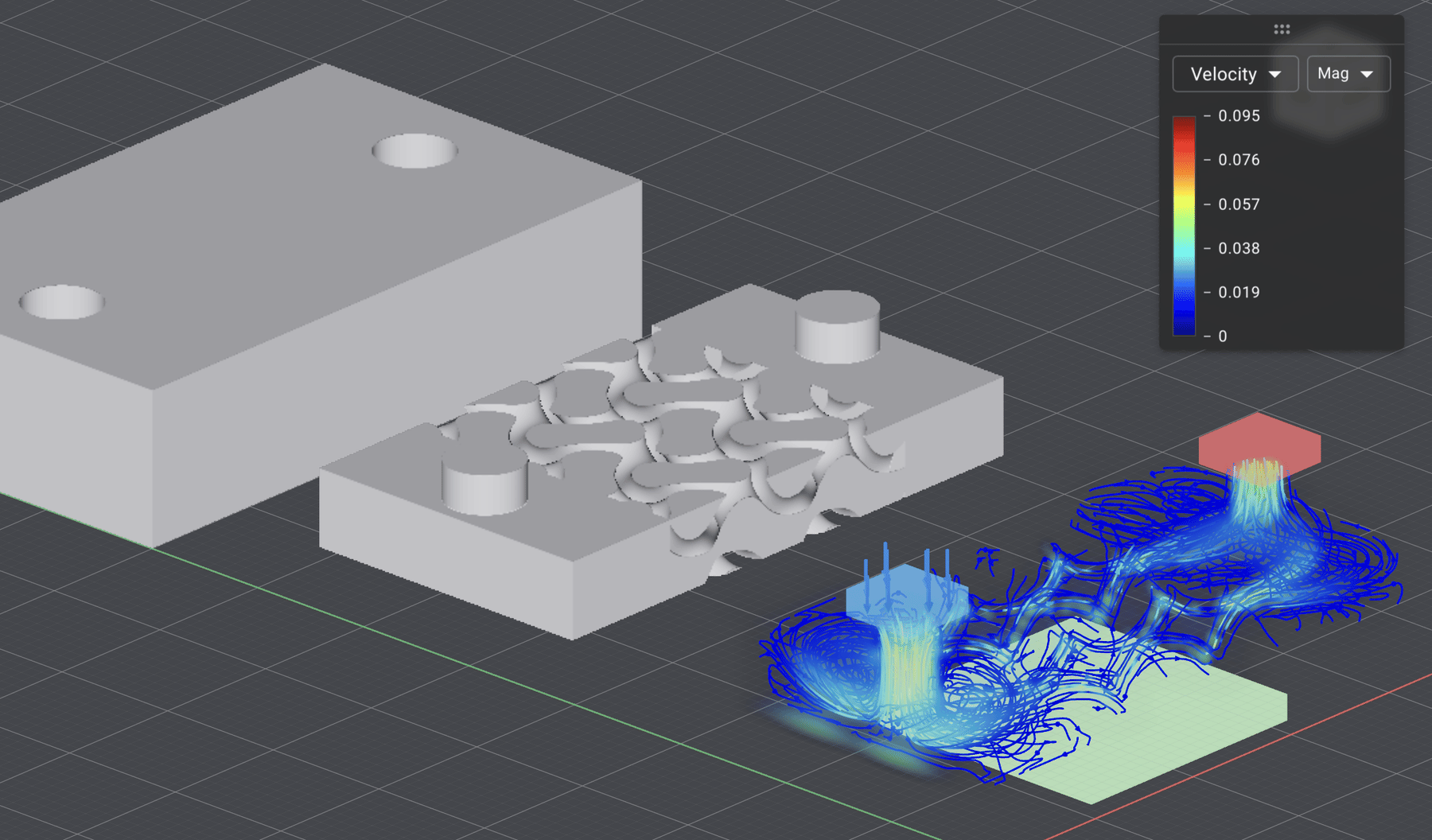
As shown in the example above, everything from shape generation to analysis setup, execution, and result visualization is contained in a single node graph, and changing a parameter re-runs the analysis as-is.
Analysis Examples
Nodi’s analysis solver can switch between multiple physics on the same input format and the same grid. Here we introduce three representative analysis types.
1. Structural Analysis
For structural analysis, linear elastic static analysis is currently supported. It solves the stiffness equation and outputs displacement, stress, and strain.
Boundary conditions are applied by specifying surfaces:
- Fixtures: displacement constraints on specified surfaces
- Loads: forces on surfaces, pressure along surface normals, moments about an axis (torsion and bending), and body forces such as gravity
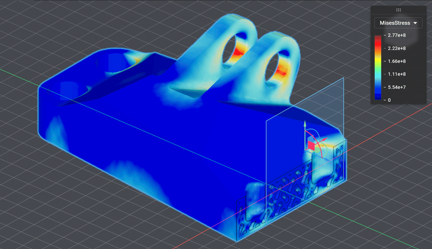
Since analysis results can be referenced directly in the node graph, this leads straight into analysis-driven shape control (field-driven design), such as “increase the lattice density only in regions of high stress”.
2. Fluid Analysis
Fluid analysis that solves the steady incompressible Navier–Stokes equations is also supported.
The “no meshing” policy applies here as well: the inside of the SDF directly becomes the fluid region, and you can start an analysis just by specifying inlet and outlet openings as surfaces.
In addition to evaluating pressure loss and velocity distribution in flow channels, conjugate heat transfer (thermal-fluid analysis combined with the thermal analysis described below) is also supported.
3. Thermal Analysis
Steady-state heat conduction analysis applies boundary conditions such as fixed temperature, heat flux, and convection on surfaces, and solves for the temperature distribution. In addition, thermal stress analysis is supported, which passes the resulting temperature field to structural analysis as a thermal strain load, allowing you to evaluate how the shape deforms and where stress arises due to temperature differences — all in a single analysis.
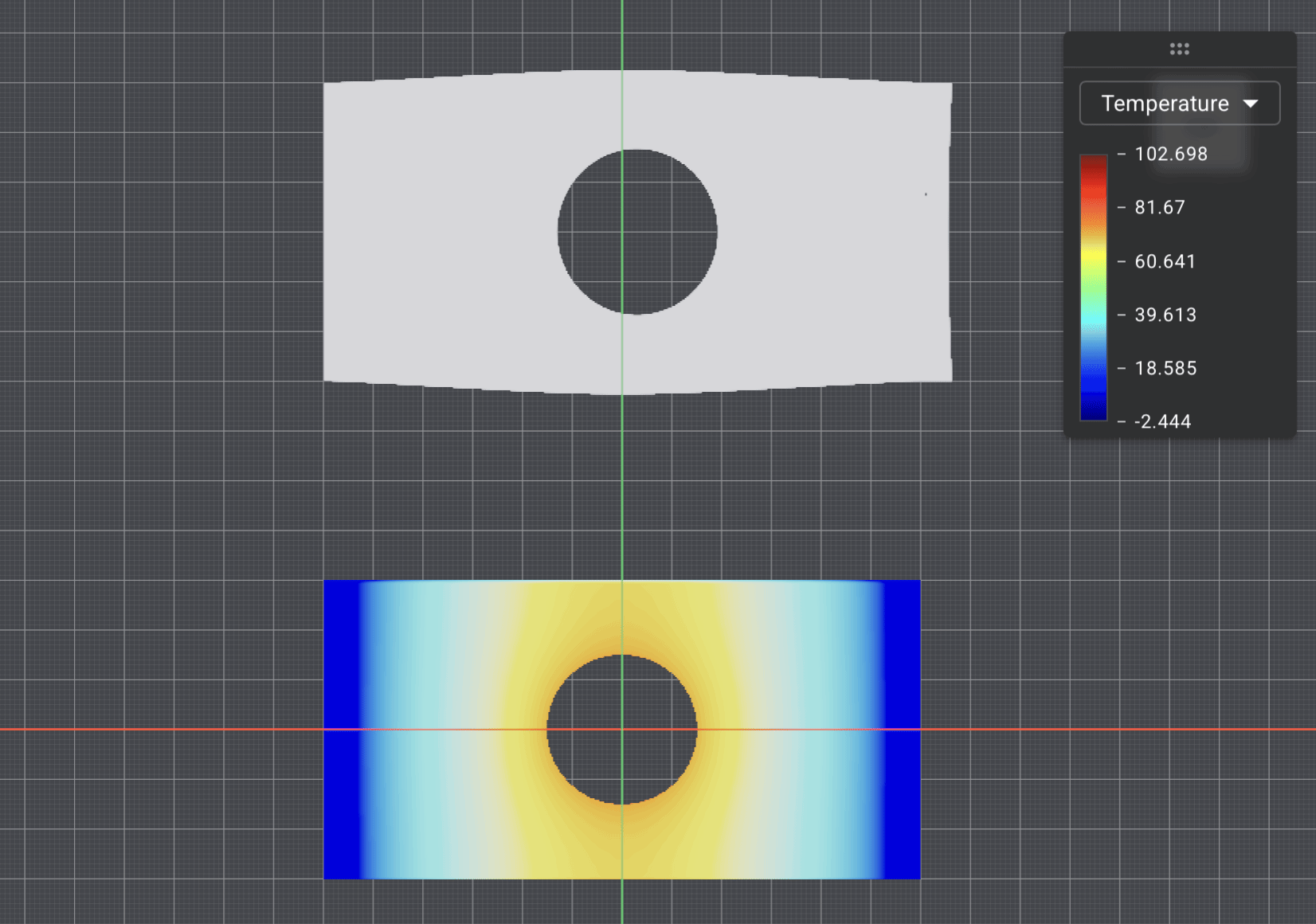
Below is an example of thermal stress analysis. The center of a plate with a hole is heated while both ends are held at a low temperature; the temperature distribution is solved (bottom), and the plate’s deformation due to thermal expansion from that temperature field is visualized (top).
Beyond this, thermal-fluid analysis (conjugate heat transfer) is also supported, coupling with fluid analysis to solve situations where “coolant in a channel cools a heat-generating solid”. This analysis menu connects directly to the thermal design domains where AM excels: heat-dissipating parts, heat sinks, molds with cooling channels, and heat exchangers.
On the Accuracy of Meshless Analysis
“If you analyze without cutting a mesh, is the accuracy really okay?” — a natural question to ask.
Nodi’s solver incorporates stabilization techniques to maintain accuracy near boundaries, and we validate it against benchmark problems with analytical solutions.
As a representative example, the tip deflection of a cantilever beam deforming under its own weight (a square-section steel bar) is compared below against the theoretical value from Euler-Bernoulli beam theory, .
| Grid resolution | Elements | Tip displacement [m] | Difference from theory |
|---|---|---|---|
| 80 × 4 × 4 | 1,280 | −2.177e-4 | 3.65% |
| 160 × 6 × 6 | 5,760 | −2.230e-4 | 1.31% |
| 240 × 8 × 8 | 15,360 | −2.243e-4 | 0.76% |
| 320 × 10 × 10 | 32,000 | −2.247e-4 | 0.54% |
The error decreases monotonically as the grid is refined, showing that accuracy can be ensured by increasing the resolution. In other words, you can quickly grasp trends with a coarse grid and raise the resolution where verification matters — all by adjusting a single parameter. The results also agree closely with those obtained by solving the same problem with conventional FEM input (explicitly specified nodes and elements), and for fluid analysis, a standard benchmark of fully developed flow in a rectangular duct shows errors below 1% against the analytical solution for both pressure gradient and centerline velocity.
Topology Optimization
Another major application of meshless analysis is topology optimization.
Topology optimization is a method that “computes the optimal material distribution under a given design space, boundary conditions, and volume constraint”. It is generally solved by updating the material distribution on a fixed grid, which makes it a natural fit for Immersed FEM, where the shape is embedded in a fixed background grid — the setup used for regular analysis (grid and boundary conditions) can be reused directly in the optimization loop.
The density field or similar output obtained from the optimization can be used directly as input to Implicit modeling, making it easy to continue into post-processing (shelling, lattice control).
1. Structural Topology Optimization
For structures, topology optimization based on volume-constrained compliance (stiffness) minimization is supported.
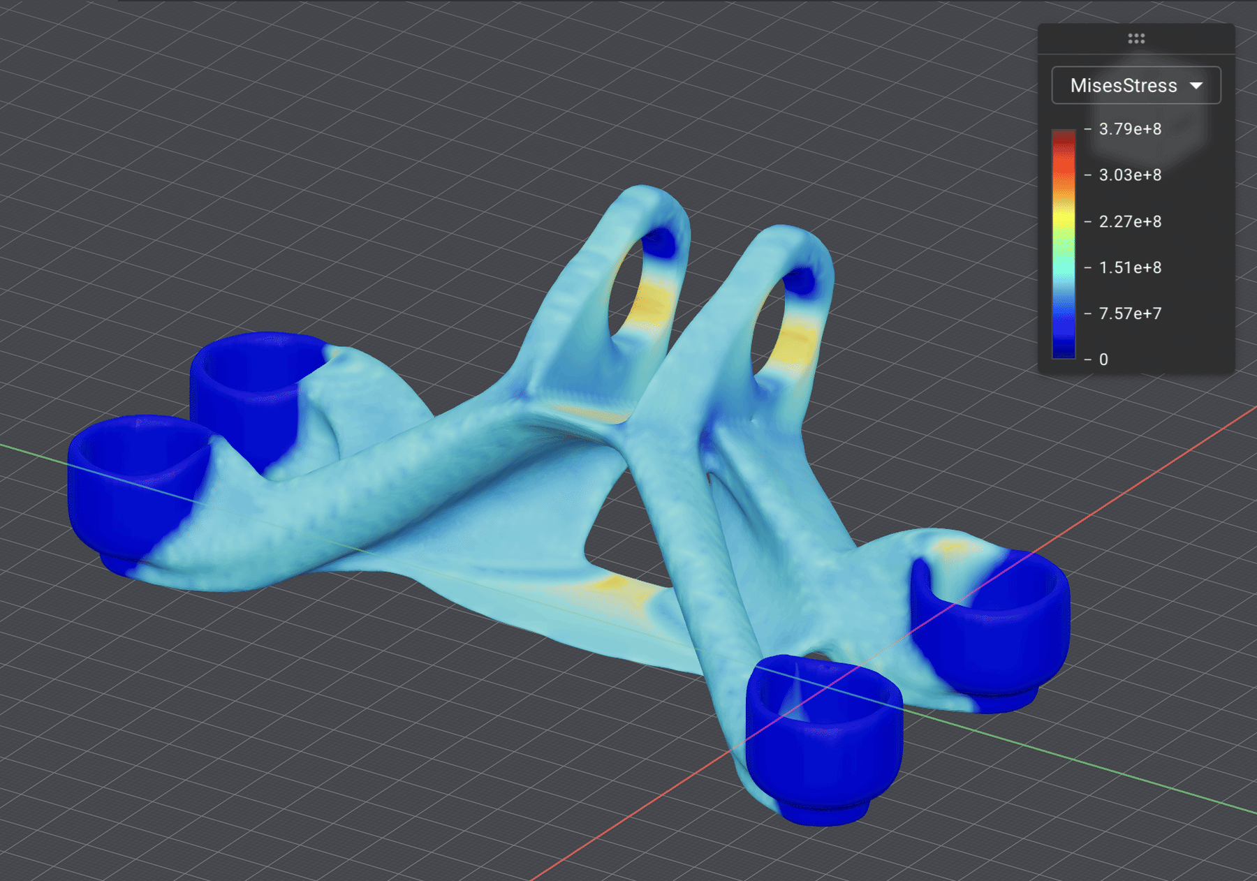
Below is a bracket example. With the four corner bolt bosses fixed and loads applied to the two upper holes, compliance is minimized under a volume constraint. An organic, branch-like structure that carries the load from the loading points to the fixtures forms automatically, and the stress distribution of the resulting shape can be checked directly.
Beyond compliance minimization, the following objectives and constraints are also supported:
- Maximum stress minimization: shape exploration aimed at suppressing stress concentration
- Heat dissipation path optimization: forming dendritic high-conductivity paths that carry heat from heat-generating regions to cooling surfaces
2. Thermal-Fluid Topology Optimization (WIP)
Currently under development is thermal-fluid (cooling channel design) topology optimization.
This uses the thermal-fluid analysis (conjugate heat transfer) introduced above as the state equation, and optimizes the very shape of the channel that most efficiently cools a heat-generating solid. Since pressure loss (pumping power) and cooling performance are in a trade-off relationship, the channel network is designed with formulations such as minimizing temperature under volume and pressure-loss constraints.
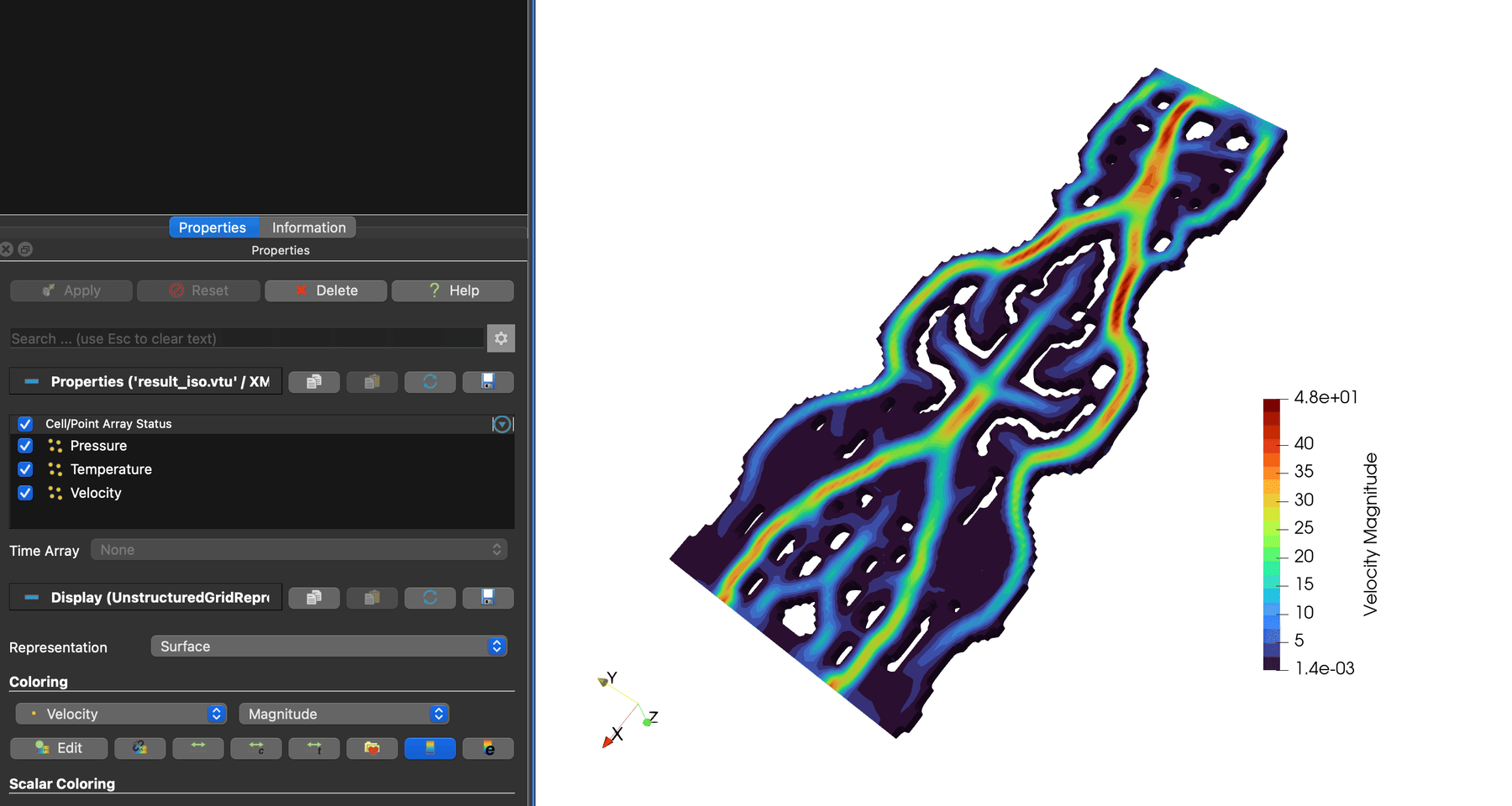
In our internal experiments, starting from a simple rectangular design domain, a vein-like branching channel network that connects the inlet and outlet while extending branches into the heat-generating region forms automatically.
This feature is still under development (WIP), but we envision applications to products where channel geometry determines performance: cooling channels in molds, power electronics cooling, and heat exchangers. By combining free-form channel geometries only AM can produce with the optimization to design them, we plan to support the DfAM workflow from the analysis side as well.
Summary
We introduced the meshless analysis (Immersed FEM) supported in Nodi.
- No meshing: shapes are embedded into a background structured grid as SDFs, and the meshing step itself does not exist
- Direct connection with Implicit modeling: even complex shapes like lattices can be passed to analysis as they are
- Extension to topology optimization: in addition to structural optimization, thermal-fluid (cooling channel) optimization is under development
By removing the meshing bottleneck that has stood between shape design and analysis, the design loop can be iterated at high speed.
If you’re interested in the Nodi desktop version, please register for the waitlist. We also welcome feedback on the analysis features and inquiries about collaboration.
Footnotes
-
Non-boundary-conforming analysis — performing analysis on a background grid that does not conform to the boundary — encompasses a variety of methods with different formulations, such as Immersed FEM, the immersed boundary method, the Fictitious Domain method, CutFEM, and the Finite Cell Method. In this article, without distinguishing between them in detail, we refer to the approach Nodi adopts as “meshless analysis (Immersed FEM)”. Note that we use “meshless” in the sense that the user does not need to prepare a mesh — this is different from so-called meshfree (particle) methods such as SPH. ↩